Business Cycle Sector Timing
The business cycle is a pattern that captures changes in economic activity over time. The changes in the business cycle occur in a sequential or serial manner, moving through a predictable sequence of phases. These cycles are consistent but vary in both duration and intensity. The phases of the business cycle are:
- Expansion: This is the phase where the economy is growing. During an expansion, economic growth is positive, leading to increased production, job creation, and rising prosperity
- Peak: The peak is the highest point in the business cycle, where the economy is operating at or near its full potential. Economic indicators may start to show signs of slowing growth, but it’s still a time of relative prosperity.
- Contraction (Recession): After the peak, the economy starts to slow down. This phase is known as a contraction or recession. Economic growth becomes negative or significantly slows, leading to reduced consumer spending, lower business investments, job losses, and declining production. This is generally a period of economic hardship.
- Trough: The trough is the lowest point in the business cycle, where the economy hits bottom. Economic indicators may show very weak performance during this phase.
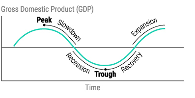
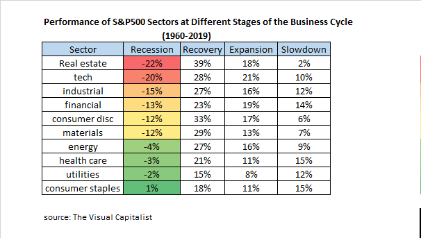
Notice that the Peak and Trough are followed by a Slowdown and Recovery. This part is important because peaks and troughs (tops and bottoms) are only known after the fact. Most of the time in the business cycle is spent in the four phases of Recession, Recovery, Expansion and Slowdown. It is logical to assume that different sectors of the economy will perform better in these four phases since they have different degrees of economic sensitivity. The original post in The Visual Capitalist was an amazing summary of S&P500 sector performance during these periods of the business cycle going all the way back to 1960. The data is summarized below:
Clear and predictable patterns begin to emerge and it is even more helpful to summarize the sector performance using normalized z-scores showing the deviation from average sector performance on a scale from 0 to 100% during each phase:
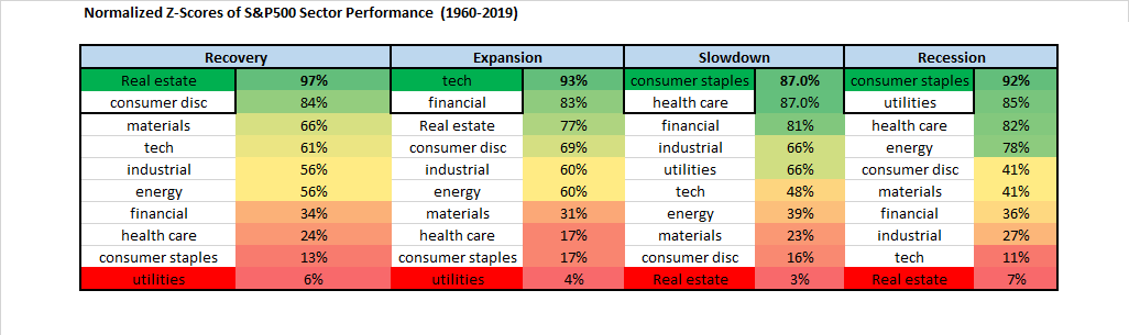
Recessions and slowdowns favor holding consumer staples which makes sense because they are products that people buy regardless of the state of the economy such as food and cleaning products. Recoveries (and also expansions) favor real estate likely due to the fact that it has more debt and hence leverage (and therefore earnings operating leverage) to a rebound in economic activity. As economic activity rebounds vacancies begin to shrink, demand causes rents to climb and the price of land and buildings also tend to rise. During expansions the fastest growing companies are naturally going to be technology companies because they are the easiest business models to scale quickly and gain millions of consumers with the least amount of capital invested.
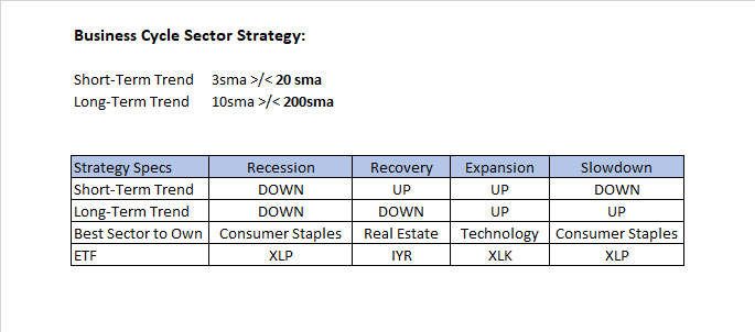
But how do we capture this in a quantitative strategy? Notice that timing the business cycle with four phases looks a lot like a trend-following strategy since we are following changes in GDP. One of the best ways to capture market expectations for changes in GDP in real time without using lagging data is to simply look at the S&P500 index. An expansion is naturally a period when both short and long-term trends are going up. A slowdown is when the long-term is up but the short-term is rolling over. A recession is when the long-term and short-term are down. A recovery is when the long-term is down but the short-term is up. This simple definition avoids having to define the four phases in economic terms but most importantly because it is impossible to predict when these phases will happen until after the fact. Every single phase of the business cycle MUST occur following changes in the trend of the market. While false signals are to be expected, this approach will be able to profit from changes that occur the few times that the signals are correct. Here is a simple strategy to capture this below:
Here is the performance of this strategy over the last 23 years. It would be interesting to see how this performs going further back using either daily or monthy data.
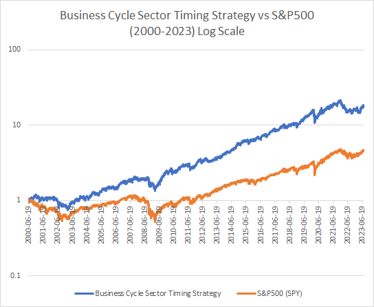
Here are the impressive summary stats of this strategy which is 100% always in the market holding equities:
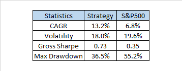
The performance of this business cycle sector timing strategy substantially outperforms the S&P500 with lower volatility. Perhaps with tactical overlays the risk-adjusted performance can be further enhanced. Having tested a lot of momentum strategies on sectors with disappointing returns the explanation is likely that they capture a lot of noise and fail to capture economic logic. There are a lot of possible ways to improve this business cycle strategy and also ways to make it more robust. Next week when I return from vacation I will try to post a follow up showing different ways to implement this strategy and also present some additional ideas. In the meantime I will not be responding to comments.
Adaptive Momentum on Major Asset Classes
In the last post on Adaptive Momentum I presented a backtest on the S&P500 via SPY. Since this was an exploratory post, I had not tried the methodology on other asset classes. I wasn’t sure how effective it would be on markets such as commodities since the leverage effect was less likely to be present. I was also curious to see how the indicator would perform on bonds and international equity markets. The results showed once again that adaptive momentum was a more profitable approach than traditional methods which was encouraging. The data tables are presented below:


Overall the results are very encouraging. Some experimentation shows that significant improvement can be made with parameter optimization and that a broad range of parameters perform quite well (default settings were by no means optimal). I like this approach as it allows for a more flexible momentum response. In contrast using fixed lookbacks or all lookbacks in a portfolio didn’t seem to address the basic issues associated with adapting to market speed. The signals for using this methodology will be added to the Investor IQ website at CSS Analytics at some point in the near future for hundreds of tickers. The performance of existing analytics on this site this year has been outstanding so this is just another tool to use. If you haven’t already joined please subscribe to this free resource using your email address.
How Should Trend-Followers Adjust to the Modern Environment?: Enter Adaptive Momentum
The premise of using either time-series momentum or “trend-following” using moving averages is the same only the math differs very slightly (see Which Trend Is Your Friend? by AQR): using some fixed lookback you can time market cycles and capture more upside than downside and therefore improve performance vs buy and hold OR at the very least improve return versus downside risk. The problem lies in the “fixed” portion of the description: markets as we know are non-stationary and business cycles can vary widely.
In 2020, the COVID-19 selloff was unprecedented in its speed and ferocity relative to past corrections. The chart below from “Towards Data Science” shows a comparison of the drawdown depth and number of days it took to get near the bottom.

What you can also gather from the chart above is that corrections in 2015 and 2018 were also relatively fast selloffs and that this may be a defining feature of the modern environment. One can speculate rationally as to the cause of this situation; monetary policy driven asset bubbles via low interest rates that artificially inflate assets like balloons that expel quickly when the air is removed, and/or computerized trading that take advantage of sellers by moving prices rapidly away as pressure increases. Regardless of the reason, the reality is that markets seem to take the escalator up and the elevator down in today’s day and age. Traditional methods that rely on linear and static time-based lookbacks have been doing quite poorly which is not surprising. An article chronicling the struggles of trend-followers was posted on Bloomberg

As you can see CTA’s have not been having an easy ride as of late and their struggles seemed to start around 2015. I know what some of you are thinking: tactical long-only trend-following with ETFs is not the same as long/short hedge funds that trade futures. You are right and wrong: right in the sense that long only ETF has a tendency to profit from asset class positive drift, whereas long/short has no such favorable tailwinds especially with low interest rates. But wrong in the sense that this doesn’t discount the timing component of returns which has been unfavorable for equity indices. The problem is more straightforward when you consider how trend-following generates excess returns. In a fantastic post by Philosophical Economics he illustrates exactly what is responsible for trend-following P/L:

The bottom line is that if markets are moving faster than the moving average oscillation period (roughly half the lookback) then you will lose money via whipsaw. This is made worse if the oscillation period is asymmetric such as when it takes longer to go up than down. Most trend-followers or tactical managers employ a 1-year or 6-month lookback. These can be too long if the drawdown materializes within less than a quarter. Furthermore using holding periods that are monthly rather than daily inspection also introduces more luck into the equation since drawdowns can happen at any time rather than on someone’s desired rebalancing period. Savvy portfolio managers use multiple lookbacks and holding periods in order to reduce the variance associated with not knowing what the oscillation period will look like. However this does not address the core problem which requires a more dynamic or nonlinear approach.
In a recent paper by Garg et. al called “Momentum Turning Points” they explore the nature of dynamic trend-following or time-series momentum strategies. They call situations where short-term trends and long-term trends disagree to be “turning points” and the number of these turning points determine trend-following performance. AllocateSmartly provides a fantastic post reviewing the paper and shows the following chart:

A greater frequency of turning points is consistent with a faster oscillation as described by Philosophical Economics. As you can see when the number of turning points increases performance tends to decrease for traditional trend-following strategies which tend to rely on longer term and static lookbacks.
Garg. et al in the paper classify different market states that result from short-term versus long-term trend-following signals:
Bull: ST UP, LT UP
Correction: ST DOWN, LT UP
Bear: ST DOWN, LT DOWN
Rebound: ST UP, LT DOWN
In reviewing optimal trend-following lookbacks as a function of market state the paper came up with an interesting conclusion:
“The conclusion from our state-dependent speed analysis: elect slower-speed momentum after Correction months and faster-speed momentum after Rebound months“
Unfortunately their solution to make such adjustments relies on longer-term optimization based on previous data. Even if this is walk-forward there is a considerable lag in the adjustment period. There is a simple way to account for oscillations that may occur more rapidly and potentially in a non-linear fashion. To state the obvious the concept of a “drawdown” is itself a nonlinear variable that is independent of time and is the most directly tied to investor profits which makes it a good candidate for making adjustments. Furthermore small drawdowns (corrections) based on the analysis presented in the paper above require longer lookbacks, while large drawdowns (that precede rebounds) require shorter/faster lookbacks. If we can use a relative measure of historical drawdowns within an adaptive framework this should more directly solve the problem. In this case we don’t care about how many turning points there are (which is the assumption made by choosing a static lookback) but rather how to adjust to them in a logical way.
The Simple Solution
The first step is to create a series of drawdowns from all-time highs (it isn’t critical to choose all-time, 1-year highs work well too). Then find the empirical distribution of such drawdowns using some lookback using a percentile ranking over the past 6 months (again not critical can use longer or shorter or a combination). I use the square of this value for the simple reason that we want to ignore small drawdowns and focus on larger drawdowns to make lookback length adjustments (remember corrections require long-term lookbacks and rebounds after large drawdowns require short-term lookbacks). Next choose a short-term trend-following lookback and a long-term lookback. In this case I chose 50 and 200 which are often followed by market participants via their respective moving averages but again the parameter choice is not critical. One practical point is that it is inefficient to use a really short-term lookback for tactical trading such as 20 days. We can calculate the optimal alpha of a moving average using the exponential moving average framework as follows:
Percentile Ranking of Drawdowns ^ 2 (squared) = P
Short- Term Alpha= ST
Long-Term Alpha= LT
Optimal Alpha= P*ST+(1-P)*LT
We then calculate an adaptive moving average using the optimal alpha which looks like this:

Notice that the adaptive moving average gets slower as the market makes new highs and faster after large drawdowns exactly as we would expect. The result is that it permits both earlier exits and entries into the market. The latter is far more important given the tendency for the market to make “V-shaped” recoveries. But to test this theory we need to backtest over a long time period and compare to traditional static lookbacks. Instead of using fixed holding periods we will do daily signal generation at the close. Since an adaptive moving average is not as effective as a simple moving average as a low pass filter it is important to filter the price when using a traditional price vs moving average strategy. To filter price I take the 10-day moving average of price (could be 3 could be 15 doesn’t matter that much). Note that the price (or filtered price) vs moving average in an exponential moving average framework is mathematically equivalent to momentum. Therefore using a price vs ema in this context is basically an adaptive momentum calculation. Here is what Adaptive Momentum looks like vs typical static lookbacks:

And for the quants out there here is the performance table:

Adaptive Momentum is the best performer in terms of CAGR, but most the biggest difference is in risk-adjusted returns (sharpe) and higher moments (skew and kurtosis). Adaptive Momentum has more positive skew and lower kurtosis indicating higher upside/downside capture and lower tail risk. What is most impressive is that it does so with nearly the same number of trades as 12-month time series momentum. If you look carefully at the line chart you can see that Adaptive Momentum does much better in recent years than the static lookbacks which we would expect. Overall performance is impressive and this can be considered as a practical approach for tactical asset allocation. An interesting note is that if you dispense with the percentile ranking in the calculation and simply increase the lookback to the maximum when the market is making new highs, and decrease the lookback to the minimum when the market is not making new highs you get pretty similar performance. Overall, the strategy doesn’t exhibit much parameter sensitivity at all.
While this simple solution is not a perfect approach, it certainly does make intuitive sense and produces worthwhile results. Given a choice between static and adaptive/dynamic I would personally take this type of approach for real-life trading.
Mean-Reversion Trading Strategies in Python Course
This post contains affiliate links. An affiliate link means CSSA may receive compensation if you make a purchase through the link, without any extra cost to you. CSSA strives to promote only products and services which provide value to my business and those which I believe could help you, the reader.
In the last post I interviewed Dr. Ernest Chan who is the author of the Mean-Reversion Trading Strategies in Python Course that I will be reviewing in this post. Readers interested in enrolling in the course can follow this link and receive an additional 5% off by using the coupon code: CSSA5
The course is put together by Quantra/QuantInsti which provides algorithmic trading courses in a slick e-learning format for a wide variety of different topics including Momentum Trading Strategies which I covered in a previous post.
Review of Mean-Reversion Trading Strategies in Python

A long time ago when I first started trading using quantitative methods, I tried implementing statistical arbitrage strategies with a friend of mine using only an Excel notebook with a data feed. While I had a reasonable understanding of what to do, I didn’t have either the technical knowledge, practical experience, or programming/operational skills to do things properly. While the backtests look great, real-life trading made them look like a mirage in an oasis. Not surprisingly, this “half-assed” operation was a failure. If only I could have gone back in time and taken this course I probably would have had a much better chance of succeeding. The course teaches you both beginner and advanced stat arb techniques and shows you how to work with Python code and connect directly to Interactive Brokers.
The course teacher- Dr. Chan- is not some ivory tower academic or financial economist discussing arbitrage opportunities on paper or the classroom chalkboard, he is an actual hedge fund manager with a successful track record. As a result the course incorporates all the important reality-checks; from the obvious such as transaction costs, to the often overlooked such as considering short-selling availability and borrow costs, to the arcane such as importance of having non-negative weights in index arbitrage to avoid added exposure via stock specific risk. In my opinion this is why quants should strongly consider taking courses on Quantra/QuantInsti if they want to at the very least avoid beginner mistakes that cost a lot more money than the cost of taking a course.
The course starts out defining stationarity and then relates this to a mean-reversion trading strategy. Various statistical tests such as the Augmented-Dickey-Fuller (ADF) test are presented along with both the requisite mathematics as well as code for calculation in Python. Then basic mean-reversion strategies are presented such as those that use Bollinger Bands or Z-scores that can be applied to stationary time series. This is extended to creating an actual portfolio of positions and how to manage this using signals to also calculating P/L. I liked the fact that an explanation was provided for why you would use statistical tests for stationarity prior to testing trading strategies since the majority of traders move immediately to backtesting.
Dr. Chan then discusses the Johansen test as a more versatile test to ADF and shows how to use the eigenvectors calculated for a wide variety of applications. The cool stuff included how to run arbitrage for triplets (3 stocks at a time) to basket arbitrage. Half-life calculations and their applications was also an important part of the content (this is often explained poorly by many sources but not in this case). I liked that the course covered risk management and also how to deal with broken pairs- something that everyone needs to know. Guidance was also provided for the best markets for pair trading. The course concludes with cross-sectional mean-reversion strategies which have been covered a lot on this blog. Python code for everything is covered in this course as well as how to apply turnkey approaches immediately in Interactive Brokers.
Overall if you are looking to get into stat arb whether at the firm level or for yourself this is a great primer. While it doesn’t show you any secret sauce, it gives you all the technical and practical coding knowledge as a foundation to developing your own. So if you are already very experienced this course probably isn’t for you. But if you are experienced but lacking in the technical/practical side you should definitely consider taking the course. There is also a Quantra community to help answer questions and build networks. Hats off to Dr. Chan and the very talented team at Quantra/QuantInsti for putting this course together.
An Interview with Dr. Ernest Chan

In the last post I reviewed the Momentum Trading Strategies Course by Quantra (a division of QuantInsti) which I reviewed as part of a recent educational journey to improve my quantitative skill set. The next course that I will be reviewing is Mean-Reversion Strategies in Python which is taught by Dr. Ernest Chan. I have personally read Ernie’s book “Machine Trading” which is very well written and full of interesting and practical ideas. I have also been a follower of his very popular blog which was a pioneer in revealing statistical arbitrage strategies such as pairs-trading. Dr. Chan is a thought leader and industry expert and anyone who is in the quantitative field has inevitably come across his work in one form or another. I reached out to interview him to get a few insights into how to think about quantitative models in the modern era. For those that are unfamiliar with Dr. Chan’s work I have provided his very impressive (and extensive) industry and educational credentials below.
Industry Background: Dr. Chan is the Founder of PredictNow.ai, a financial machine learning SaaS, and also the Managing Member of QTS Capital Management, LLC., a commodity pool operator and trading advisor. His primary focus has been on the development of statistical models and advanced computer algorithms to find patterns and trends in large quantities of data. He has applied his expertise in statistical pattern recognition to projects ranging from textual retrieval at IBM Research, mining customer relationship data at Morgan Stanley, and statistical arbitrage trading strategy research at Credit Suisse, Mapleridge Capital Management, and other hedge funds.
Educational Background
Dr. Chan is an industry expert on ‘Algorithmic Options Trading’ and has conducted seminars and lectures on many international forums. Besides being a faculty in QuantInsti, his academic distributions are available on Quantra and on major web portals. Dr. Chan is also an adjunct faculty at Northwestern University’s Master’s in Data Science program. His courses and publications on finance and machine learning can be found at www.epchan.com. Ernie is the author of “Quantitative Trading: How to Build Your Own Algorithmic Trading Business”, “Algorithmic Trading: Winning Strategies and Their Rationale”, and “Machine Trading”, all published by John Wiley & Sons. He maintains a popular blog “Quantitative Trading” at epchan.blogspot.com. Ernie received his PhD. in Physics from Cornell University.
Interview with Dr. Ernest Chan
1) What do you think about traditional factor investing and trading strategies that use technical indicators? Can they be profitable in the modern environment?
We don’t use machine learning to generate trading signals, but rather to determine the probability of profit of the existing trading signals generated by a basic, traditional quantitative strategy. This strategy can be a factor model or one based on simple technical indicators. This probability of profit can then be used to determine the order size, which can be zero if the probability is too low.
Factors and technical indicators are still crucial for the basic strategy. I don’t believe that machine learning can replace human intuition and understanding. In fact, it should be used to enhance such understanding and risk management. The input to a machine learning algorithm is nothing but factors and technical indicators.
2) If you could choose between a Momentum and Mean-Reversion approach to trading which would you choose and why?
I would trade both. Otherwise the portfolio would not be market neutral since momentum strategies are typically short beta while mean reversion strategies are long. Also, momentum strategies are long “gamma” and “vega”, while mean reversion strategies are short. Note that I put quotation marks around such options Greeks because we are not really trading options nor implied volatility. I am using these terms loosely to indicate an increase in tail movements and realized volatility.
3) Why should traders strongly consider using machine learning in their trading versus hand-coding their own quantitative systems or using more simple statistical tools? For traders that aren’t familiar with coding what do you think is the best way to get started?
Traditional quant strategies are too easily replicated by other equally intelligent traders, hence they suffer more rapid alpha decay. ML strategies have so many parameters and nuances that no two traders can possibly have the same strategy. For traders who are not experts in machine learning or programming can start with a no-code machine learning service such as predictnow.ai.
4) What do you think is the biggest challenge for newbies trying to design their own machine-learning models?
Machine learning requires abundant and correctly engineered features as input. I have seen many newbies trying to use 4 or 5 inputs to a ML algorithm. They should instead be using at least 100 inputs.
5) Do you have a preference in terms of the type of machine learning model you use such as Neural Networks vs KNN or Decision Trees? If so why?
Decision trees, or the more advanced version called random forest, is the preferred ML method for trading. That’s because it doesn’t have as many parameters to fit as a neural network, thus reducing the danger of data snooping bias. Also, the output of a decision tree is a bunch of conditional decision rules, which are much easier to interpret than the nonlinear functions that neural networks use. On the other hand, KNN or logistic regression are too simple – they don’t capture a lot of the nonlinear dependence between different input features and the output return.
6) Many traders and market commentators have noticed that markets seem quite a bit different than in the past. The market seems to move much more quickly and reacts to news in ways that are counterintuitive. Given your vast experience with algorithmic trading what new trends or insights have you gathered in the last few years? Have you made any specific adjustments or recalibrated your models accordingly?
Market patterns often deviate from the “norm” over a short period (e.g. 6 months-1 year), but they often revert to the norm. One needs to diversify so that some strategies are enhanced during such periods, even though others are hurt. Such regime changes can also be detected or predicted to some extent by machine learning.
Thanks Ernie for the interview!
Momentum Trading Strategies Course
This post contains affiliate links. An affiliate link means CSSA may receive compensation if you make a purchase through the link, without any extra cost to you. CSSA strives to promote only products and services which provide value to my business and those which I believe could help you, the reader.
One of the biggest barriers to creating a quantitative strategy is knowing how to code. The other barrier is having sufficient theoretical and empirical knowledge. Getting a degree in finance can help with the latter, and a computer science degree can help with the former but if you want to be able to do both you often have to start from scratch which can be very intimidating. I recently took the Momentum Trading Strategies Course by Quantra which is unique because it teaches you both the background theory and empirical research as well as how to code examples in Python– currently the most popular language for algorithmic traders. Given that my coding skills are limited to using Microsoft Excel, this course was especially useful and I even learned a few new things on the research side. Readers interested in enrolling in the course can follow this link and receive an additional 5% off by using the coupon code: CSSA5
Note: This course is currently priced at $179 but will return to its normal price of $499 on November 2.
Before getting to my review of the course below it is important for readers to know a little bit more about the service and the players behind the scences:
Quantra is a learning platform for algorithmic trading courses, where through advanced interactive & hands-on learning technology offers content curated by some of the top thought leaders in the domain of algorithmic trading including;
1) Dr Ernest P. Chan
2) Laurent Bernut
3) Dr Terry Benzschawel
4) National Stock Exchange (World’s Biggest Derivatives Exchange)
5) Multi Commodity Exchange (India’s Leading Commodity Exchange)
6) Interactive Brokers
7) Forex Capital Markets (FXCM)
The parent company of Quantra is QuantInsti, which was founded by one of India’s biggest HFT firms; iRage, is today one of the world’s most prominent algorithmic & quantitative trading & research institutes with a user base in 180+ countries.
Review On Momentum Trading Strategies Course
First I have to say that this is a really comprehensive course with very slick technology for the e-learning community. The course took me a couple days to complete which was longer than I expected but it also went into far greater depth than I expected as well. To get the most out of the course you should also read the recommended research articles and also work on coding the examples.
It starts off very basic- almost too basic for those familiar with momentum- but gradually builds and gets more advanced with each segment. The topics covered early on include answering what momentum is and why it exists as an anomaly. By the time you get to the fifth section you are being introduced to Python and how to work with commands and loading in data for analysis. You then cover more advanced topics like how to use the Hurst Exponent to cross-sectional arbitrage strategies in futures that exploit roll returns.
In this comprehensive curriculum it seems like every major popular paper on momentum is neatly summarized and the course also covers important topics like Momentum Crashes and risk management. Each segment has examples linked to using Python. There are also multiple choice questions that are there to test your memory and comprehension of the material. As you reach the end of the course you are introduced to even more practical topics like how to automate trading strategies and link to broker APIs.
Overall I was very impressed and I think this is exactly the kind of e-learning alternative that both students and traders/investors need to make their dreams of having their own automated strategy a reality. In subsequent posts I plan to continue to share my learning journey by trying new courses and will provide readers again with a review. Hats off to the team at QuantInsti for being an innovator in this space.
Adaptive VIX Moving Average with Ehlers Alpha Formula
In the last post I described a relatively simply method to incorporate the VIX into the well-known AMA or Adaptive Moving Average framework. The alpha formula requires two separate parameters- a short and a long-term constant which requires greater specification by the user. Ideally the fewer parameters you have to specify the better (although it is important to note that logical requirements for maximum lag and minimum responsiveness often tends to dicate the bounds).
Ehlers suggests in his paper on the “Fractal Adaptive Moving Average” using the following formula to compute the alpha in the exponential average:
alpha= exp(- 4.6*(D -1))
where D is analogous to the “VI” or trend factor in the previous post. Note that this formula was adapted in a different way for creating an adaptive volatility measure in this post. I find it to be quite useful and intuitive so it represents a viable alternative to the AMA framework in the last post.
Based on reader feedback I will simplify the percentrank function to be a rolling lookback of 2000 days to make it easier to avoid confusion in replication (the previous used an anchored lookback or “expanding time window”). We can substitute the percentrank of 1/(10-day sma of VIX) for “D” in the formula and calculate the EMA/Exponential moving average of SPY using the alpha output. Here is what the adaptive alpha should look like going back to 1996:

Note that a higher alpha means a faster moving average (less smoothing and lag) while a lower alpha means a slower moving average (more smoothing and lag). We can see in the above chart that the alpha is higher most of the time in bull markets and lower in bear markets (with the 90’s being an exception). No doubt there is a relationship between the VIX and mean-reversion which tended to work well on SPY in periods when the alpha was low. My research in fact shows that profitability was 4x higher buying on down days when this alpha measure was low versus high. What this implies is that you are smoothing more when price is noisy or mean-reverting and smoothing less when price is a decent estimate of tomorrow’s price. Obviously this is exactly what we are looking for when creating an adaptive filter.
Let’s now take a look at how this new transition calculation performs in the adaptive moving average framework. Once again we will compare the strategy of buying when the close of SPY is > 200sma versus the AMA> 200sma.
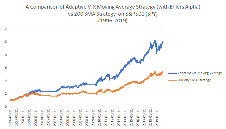

Consistent with the previous post the AMA strategy is superior to the basic 200sma strategy with fewer trades. The Ehlers alpha method in this case leads to very similar results as using the classic AMA framework for calculating alpha but with even fewer trades. Note that a “D” of 4 vs 4.6 produced a near identical match to the performance and number of trades as the classic AMA framework. In either case I hope this shows the robustness of using the VIX (or you could use historical volatility or GARCH) in an adaptive moving average as a substitute for using the price. In my opinion it is logical to use an adaptive method for smoothing rather than using static smoothing methods or worse yet the actual price in a trend-following strategy.
Adaptive VIX Moving Average
One of the challenges with technical or quantitative analysis is to identify strategies that can adapt to different market regimes. The most obvious is a change in the forecast or implied volatility as proxied by the VIX. During more volatile periods we would expect more signal noise and during less volatile periods we would expect less signal noise. But how do we capture this in a strategy? One method is to use the VIX to standardize returns as presented on this blog used “VIX-Adjusted Momentum” in this post. An excellent recent follow-up analysis was done by Justin Czyszczewski which showed that VIX-adjusted trend-following has been recently very successful during these fast moving markets (Tip: using the median or average of O,H,L,C of VIX versus closing data will make the edge of the original strategy more consistent across history). I will show a new variation using this framework very soon in a follow-up post.
Another way to tackle this issue is to vary the lookback length as a function of the VIX. So how would we do that? Enter the basic adaptive moving average framework which seeks to vary the speed or lookback of the moving average as a function of some volatility or trend-strength function.

We can easily substitute the VIX within the “VI” by looking at a standardized measure of how high or low volatility has been relative to past history. If it is higher we want to smooth more or have a longer lookback, and if it is lower we want to have a shorter lookback. This can be accomplished as follows:

Basically we are taking the percentile ranking using all history to date of 1 divided by the current average VIX over the past 10-days. To visualize how this moving average works we can see it applied to the S&P500 (SPY) in the chart below:

Notice that the moving average tracks the price very closely during bull markets and then filters out noise by becoming smoother during corrections. This is exactly what we want to see! Now lets compare a standard 200-day sma strategy that uses the current price versus using the Adaptive VIX Moving Average filter.
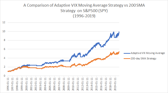
The result is a nice boost in gross performance (no transaction costs) that also happens to come with far fewer trades (48 vs 164) which would even further boost net performance. The results are in the table below:
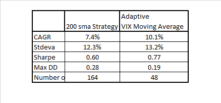
This concept can be extended in several ways including using a simple moving average on the AMA line to create faster crossover strategies that are more responsive to market conditions. Ultimately this is a very simple and intuitive way to adjust standard trend-following as a function of changing volatility regimes.
Which Quant ETFs are Outperforming?
One of the challenges of investing in today’s environment is that there are so many investment products that it is hard to keep track. Our recently launched site Investor IQ is designed to help better organize investors and provide them with the analytics required to make better decisions. The biggest risk to chasing performance is if you aren’t on top of what is happening now and instead are chasing the last 3-year or 5-year winning fund (which are likely to mean-revert). Our relative strength rating tracks momentum at shorter intervals in order to better capture future outperformance. Here is a current snapshot of our “Quant ETFs” category under US ETF Digest which makes it easy to see which quant styles are outperforming right now:

As you can see the market is currently favoring stocks that are either undervalued (Value Screen/QVAL and Shareholder Yield/SYD) or exhibit growth at a reasonable price (GARP) which are ranked at the top by relative strength or “RS Score”. This reflects a significant shift away from growth (FFTY) and momentum (QMOM) which are ranked in last place. In fact the signal- which an ensemble of trend and momentum signals- shows that their trends are in a caution or “Hold” position while all other factors remain in a “Buy” signal. The OB/OS oscillator in the far right column is an ensemble of mean-reversion indicators that ranges from 0 to 100 (least to most overbought). Currently all of the ETFs in the list are neutral in terms of timing but nearing overbought territory (>80) where new purchases should either be avoided or existing positions should be trimmed.
The goal of this list was to capture many of the factors that quants use to produce alpha versus the broad index in a long-only format. We deliberately omitted strategies that had the ability to raise cash since I would consider that a separate genre of tactical strategies. If you have suggestions for additional quant ETFs that are not redundant to the members of this current list feel free to leave them in the comments section and I will seek to add them over time pending review.
Investor IQ Website is Live (In Beta)
For readers interested in getting signals and analytics on hundreds of ETFs and individual stocks our Investor IQ website is currently live and free during our beta-testing phase. We will be adding new data and analytics gradually over time as well as improving website functionality. The Economic Model is currently hosted on the site and predictions are updated every 2-3 days in real-time. Subscribers will soon receive access to backtests on the economic model (I have received plenty of requests) and other research unique to the website. For the time being we will continue to publish Investor IQ on this blog with limited functionality on a weekly basis for our readers so be sure to sign up to the website as soon as you can!

